This article presents some Python code for computing the log-likelihood of a sample under a multivariate Gaussian distribution, along with the formulas used to justify the method of computation.

The One-Dimensional Case

The likelihood of a data set under a Gaussian model can be computed using only the sample mean, sample variance, and sample size of the data set, as follows:

import numpy as np

def logpdf(sample_mean, sample_variance, sample_size, mean, variance):
    """ Compute a Gaussian log-density from statistics. """
    relative_sample_variance = sample_variance / variance
    relative_meandev2 = (sample_mean - mean)**2 / variance
    logdet = np.log(2 * np.pi * variance)
    nlogptwice = logdet + relative_sample_variance + relative_meandev2
    return -0.5 * sample_size * nlogptwice

You can verify this code by comparing the output of

logpdf(np.mean(x), np.var(x), len(x), mean, variance)

to

scipy.stats.norm.logpdf(x, loc=mean, scale=scale).sum()

This method of computation relies on the fact that

$$\sum_i \left( \frac{x_i - \mu}{\sigma} \right)^2 = \sum_i \left( \frac{x_i - \hat{\mu} + \hat{\mu} - \mu}{\sigma} \right)^2 = \frac{N\hat{\sigma}^2}{\sigma^2} + \frac{N(\hat{\mu} - \mu)^2}{\sigma^2},$$

where \( \hat{\mu} \) the sample mean, \( \hat{\sigma}^2 \) is the sample variance, and N is the size of the data set. The formula holds because the average of the cross-terms is zero.

The p-Dimensional Case

Does a similar formula exist for the multivariate Gaussian?

The analogy with the one-dimensional cases suggests that it should possible to compute the likelihood of a sample under a Gaussian distribution using only the sample mean vector, the sample covariance matrix, and the sample size.

And indeed, that happens to be possible, as follows:

import numpy as np

def logpdf(sample_mean, sample_cov, sample_size, mean, cov):
    """ Compute multivariate Gaussian log-density from statistics. """
    invcov = np.linalg.inv(cov)
    relvar = np.trace(sample_cov @ invcov, axis1=-2, axis2=-1)
    meandiff = sample_mean - mean
    meandev2 = np.squeeze(meandiff[..., None, :] @ invcov @
                          meandiff[..., :, None])
    _, logdet = np.linalg.slogdet(2 * np.pi * cov)
    nlogptwice = logdet + relvar + meandev2
    return -0.5 * sample_size * nlogptwice

This can be verified by comparing

scipy.stats.multivariate_normal.logpdf(x, mean, cov).sum()

to

logpdf(np.mean(x, axis=0), np.cov(x.T, bias=True), len(x), mean, cov)

The justification requires an extra step in this case, though. Using the notation

$$\Vert v \Vert^2_C = v^T C^{-1} v$$

to designate the squared Mahalanobis norm of \( v \) , we can again expand

$$\begin{eqnarray} \sum_i \Vert x_i - \mu \Vert^2_C & = & \sum_i \Vert x_i - \hat{\mu} + \hat{\mu} - \mu \Vert^2_C \ & = & \sum_i \Vert x_i - \hat{\mu} \Vert^2_C + \Vert \hat{\mu} - \mu \Vert^2_C. \end{eqnarray}$$

(I realize it's confusing to use \( C \) as the subscript instead of \( C^{-1} \) , but apparently Hashnode can't cope with subscripts of more than one character.)

This formula still includes references to the particular observations in the data set, so we have not yet expressed the likelihood purely in terms of summary statistics. Fortunately, though, we can express the squared Mahalanobis distance as a matrix trace in the following way:

$$z^T M z = tr ( vv^T M )$$

This can be verified by writing out the trace on the right-hand side explicitly as a nested sum and comparing the terms to the left-hand side.

Together with the properties of the trace function, this allows us to prove that

\[\sum_i \Vert x_i - \hat{\mu} \Vert^2 = tr \left( \sum_i (x_i - \hat{\mu})(x_i - \hat{\mu})^T C^{-1} \right) = N tr(\hat{C}C^{-1}).\]

This is the formula for the relative variance used in the function.

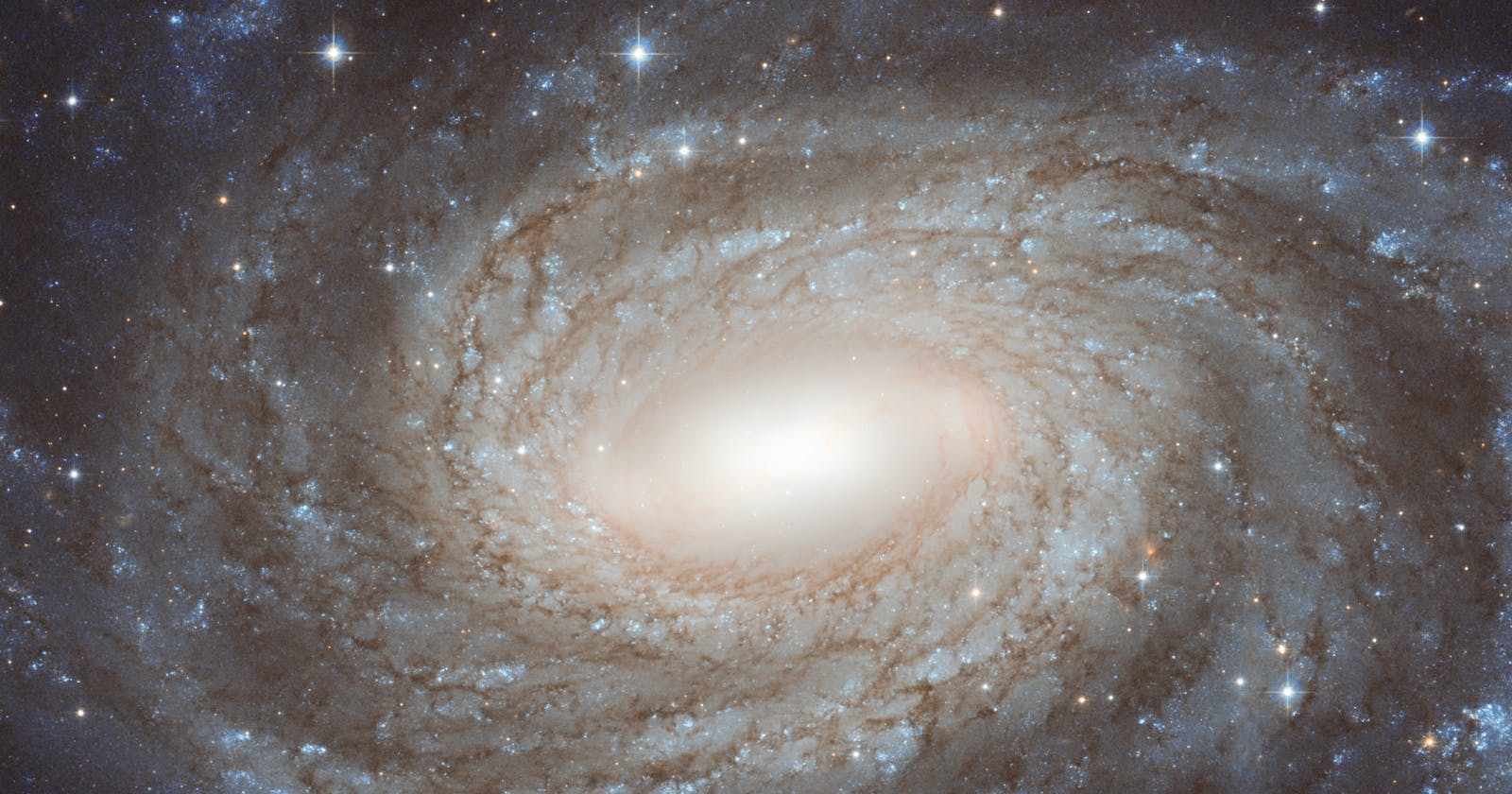
Image credits: The cover image is a photograph of the galaxy NGC 6384 taken by the Hubble space telescope. The other illustrations are by me.