Peano's space-filling curve is a uniformly continuous and surjective mapping of the unit interval onto the unit square. The curve is a fractal — it is constructed using a recursive refinement scheme that doubles its length in each iteration.

Corner-to-Corner Tiles

Here is Hilbert's illustration of the construction:

As these images suggest, the curve can be constructed by making a single large tile out of four smaller tiles (allowing rotation and mirroring of the pattern):

If the image on the tile is a curve connecting the bottom left corner to the bottom right corner, then this stacking scheme results in the composite tile also depicting a continuous curve connecting the bottom left corner to the bottom right corner:

From Tiles to Computations

Suppose you have defined a function g(t) which maps the unit interval onto a curve inside the unit square, with g(0) = (0, 0) and g(1) = (1, 0). Then the following code tiles that curve into an n'th approximation of the Peano curve:

def p(t, n=10):
    """ A point (x, y) on a recursive curve in [0, 1]^2. """
    if n <= 0:
        return g(t)
    elif 0 <= t < 1/4:
        x, y = p(4 * t, n - 1)
        return (0.5*y, 0.5*x)
    elif 1/4 <= t < 1/2:
        x, y = p(4*t - 1, n - 1)
        return (0.5*x, 0.5 + 0.5*y)
    elif 1/2 <= t < 3/4:
        x, y = p(4*t - 2, n - 1)
        return (0.5 + 0.5*x, 0.5 + 0.5*y)
    elif 3/4 <= t <= 1:
        x, y = p(4*t - 3, n - 1)
        return (1 - 0.5*y, 0.5 - 0.5*x)
    else:
        raise ValueError("Unexpected input: %r, %r" % (t, n))

The Peano curve is the pointwise limit of this function as n goes to infinity. Since it is the limit of a series of uniformly continuous curves, it is also uniformly continuous.

Finding the Visting Time

If you divide the unit interval up into four temporal segments, then the images of these four segments are four spatial quadrants of the unit square: the bottom left, top left, top right, and bottom right — in that order. If we continue to divide one of these segments up into four sub-segments, then the four sub-segments correspond to four sub-quadrants inside the corresponding quadrant.

To find a t whose image is the point (x, y), we can therefore repeatedly ask which sub-quadrant (x, y) lies within, and use this information to compute a series of increasingly good approximations of t, with each subdivision allowing us to find one additional digit in the base-4 expansion of t:

Here is code for finding the n'th lower bound in that sequence:

def tapprox(x, y, n=10):
    """ Compute a lower estimate of `t` from `(x, y)`. """
    if n <= 0:
        return 0.0
    elif 0 <= x < 1/2 and 0 <= y < 1/2:
        return 1/4*tapprox(2*y, 2*x, n - 1)
    elif 0 <= x < 1/2 and 1/2 <= y <= 1:
        return 1/4 + 1/4*tapprox(2*x, 2*y - 1, n - 1)
    elif 1/2 <= x <= 1 and 1/2 <= y <= 1:
        return 2/4 + 1/4*tapprox(2*x - 1, 2*y - 1, n - 1)
    elif 1/2 <= x <= 1 and 0 <= y < 1/2:
        return 3/4 + 1/4*tapprox(1 - 2*y, 2 - 2*x, n - 1)
    else:
        raise ValueError("Unexpected input: %r, %r, %r" % (x, y, n))

This sequence of lower bounds converges exponentially fast to a value t whose image is (x, y).

The Choice of Base Case

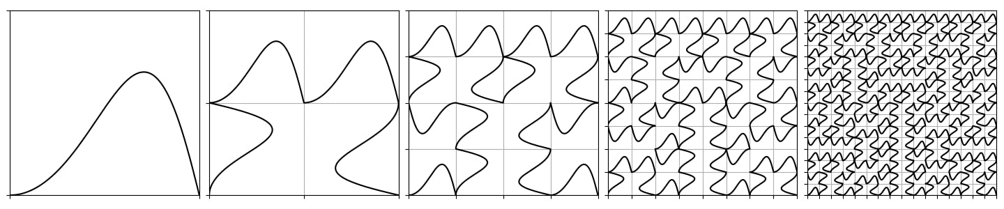
As I mentioned above, the code I provided assumes that you have defined a two-dimensional curve g(t) whose values live inside the unit square and connect (0, 0) to (1, 0). For drawing above, I used the following choice:

import numpy as np

def g(t):
    """ A point (x, y) on a curve in the unit square. """
    return (t, 2/3*np.sin(np.pi * t**2))

However, other choices are possible:

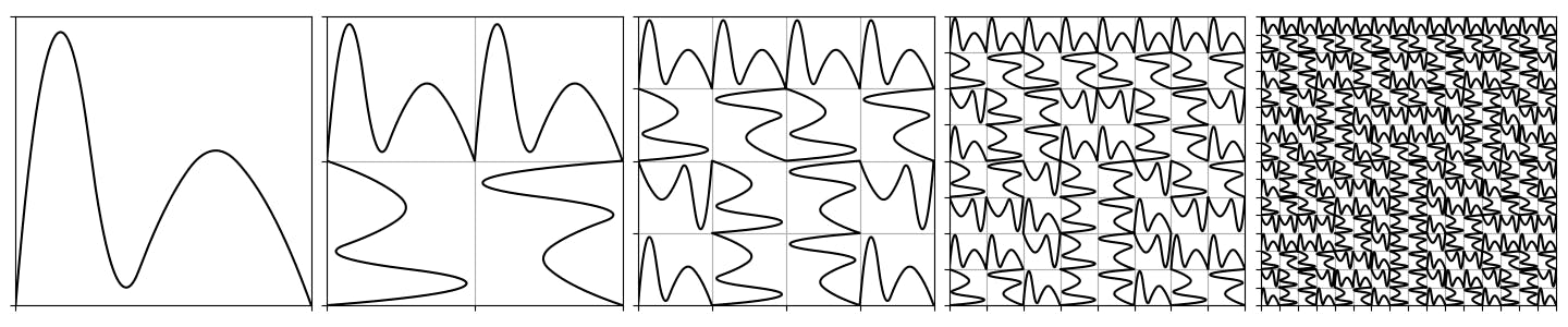
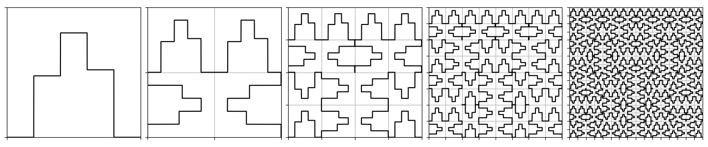
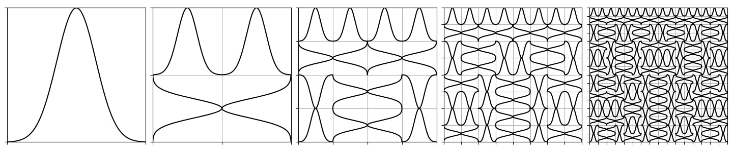
The choice of base case dramatically influences the look of the first few iterations, but its influence ultimately vanishes in favor of the recursive structure.

Image credits: the cover image and the picture of the tulip tile are from the Wikipedia article about tiles.