The t distribution has long tails and is therefore robust against outliers. If we can fit a multivariate t distribution to a data set of input-output pairs, we can therefore perform outlier-robust linear regression. This post provides code that does that.

Warning: Hashnode tends to destroy math formatting without warning, sometimes even after it successfully compiles. I've tried to make sure the formulas below are displayed correctly, but errors may have been introduced after my last reading.

The Univariate Case

Here is a piece of code that can fit a location-scale family of t distributions to data:

import numpy as np

def t_fit(x, df, niter=10):
    """ Estimate loc. and scale parameters of a t distribution. """
    weights = np.ones(len(x))
    for _ in range(niter):
        mu_hat = np.average(x, weights=weights)
        sigma2_hat = np.cov(x, bias=True, aweights=weights)
        mahalanobis2 = (x - mu_hat)**2 / sigma2_hat
        weights = (df + 1) / (df + mahalanobis2)
    return mu_hat, sigma2_hat

You can verify the soundness of this method by comparing it to

scipy.stats.t.fit(x, fdf=1)

Why does this work?

The t distribution is a mixture of Gaussians with different scale parameters. If we integrate out the random variation in the scale parameter, we obtain an explicit formula for the density of the distribution. However, we can also find the maximum likelihood parameters without performing any integration by using the EM algorithm.

Specifically, suppose the observations are generated according to the following sampling program for \( i = 1, 2, \ldots, N \) :

$$G_i \sim \Gamma(d/2, d/2)$$

$$T_i , | , G_i \sim \mathcal{N}(\mu, \sigma^2/G_i)$$

(I am using the shape-rate parameterization of the gamma distribution.)

Under this sampling program, the marginal distribution of T is a t distribution. We can find the maximum-likelihood estimates of \( \mu \) and \( \sigma^2 \) given a data set \( t_1, t_2, \ldots, t_N \) if we know how to compute

1. the maximum-likelihood estimates of \( \mu \) and \( \sigma^2 \) given fixed \( G_i \)

2. the conditional distribution of each \( G_i \) given fixed \( \mu \) and \( \sigma^2 \)

Since each \( G_i \) follows a gamma distribution, each \( V_i = 1/G_i \) follows an inverse-gamma distribution. The inverse-gamma distribution has the probability density

$$p(v_i) \propto (1 / v_i)^{d/2 + 1} \exp\left(-(d/2)(1 / v_i) \right)$$

By assumption, the conditional distribution of \( T_i \) given \( G_i = g_i = 1/v_i \) is a Gaussian with variance \( \sigma^2 v_i \) . That means its density is given by

$$p(t_i , | , v_i) \propto (1 / v_i)^{1/2} \exp\left( -\frac{1}{2v} \frac{(t_i - \mu)^2}{\sigma^2} \right)$$

The joint distribution is therefore

$$p(t_i, v_i) \propto (1 / v_i)^{d/2 + 1 + 1/2} \exp\left( -\left(\frac{d}{2} + \frac{(t_i - \mu)^2}{\sigma^2} \right) (1 / v_i) \right)$$

Considered as a function of \( v_i \) , this joint probability density is proportional to an inverse-gamma density with parameters

$$\alpha_i = \frac{d}{2} + 1$$

$$\beta_i = \frac{d}{2} + \left( \frac{t_i - \mu}{\sigma} \right)^2$$

The conditional distribution of \( G_i \) given \( \mu \) and \( \sigma^2 \) is therefore a gamma distribution with the same parameters and

$$E(G_i) = \frac{\alpha_i}{\beta_i} = \frac{d + 1}{d + (t_i - \mu)^2 / \sigma^2}$$

That takes care of the E step of the EM algorithm, computing the conditional distribution of the nuisance variables given fixed values of the parameters.

We can then move on to the M step, that is, finding the parameter values that optimize the surrogate loss

$$E_G \left( -2 \sum_i \log p(t_i , | G_i) \right) = N \log(\sigma^2) + \sum_i E(G_i) \frac{(x_i - \mu)^2}{\sigma^2}$$

Minimizing this surrogate loss with respect to \( \mu \) and \( \sigma^2 \) is equivalent to fitting the parameters of a Gaussian to a data set with observation weights \( E(G_i) \) . That is exactly what the code above does in the first two lines of each iteration. (Note that observations further from the previous location estimate have smaller weights, but that the distance matters less when d is large.)

The Multivariate Case

Can we generalize this to the multivariate t distribution? Yes, we can:

import numpy as np

def t_fit(x, df, niter=10):
    """ Estimate location vector and squared-scale matrix. """
    weights = np.ones(len(x))
    for _ in range(niter):
        # M step: optimize parameters given conditional distributions
        mu_hat = np.average(x, axis=0, weights=weights)
        cov_hat = np.cov(x.T, bias=True, aweights=weights)
        # E step: compute conditional distributions given parameters
        inv_cov = np.linalg.inv(cov_hat)
        inv_cov_x = np.squeeze(inv_cov @ x[:, :, None], axis=2)
        mahalanobis2 = np.sum(x * inv_cov_x, axis=-1)
        weights = (df + 1) / (df + mahalanobis2)
    return mu_hat, cov_hat

The justification here is exactly the same, except now we have

$$G_i \sim \Gamma(d/2, d/2)$$

$$T_i , | , G_i \sim \mathcal{N}(\mu, C/G_i)$$

where \( \mu \) is a mean vector, and \( C \) is a positive-definite covariance matrix. This describes a distribution where the radial distance from the observation to the mean is scaled by a random factor.

Here are an illustration of how this iterative method deals with a problematic data set:

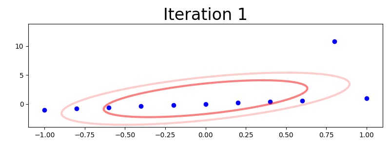
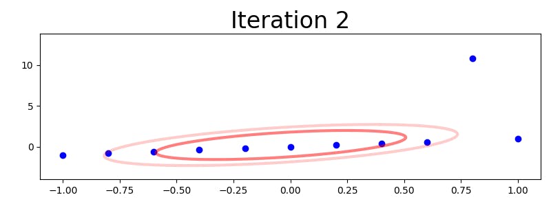
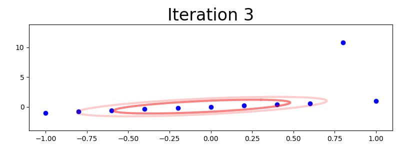
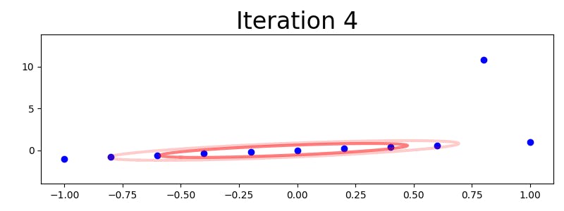
(I tried uploading an animated GIF, but Hashnode renders it has a static image.)

As the picture indicates, the algorithm quickly learns to assign a very low value to the outlier observation, so that the resulting model becomes very precise in the absence of random distance stretching. For reference, here is another example that shows the difference between fitting a multivariate Gaussian and a multivariate t distribution to a two-dimensional data set with outliers:

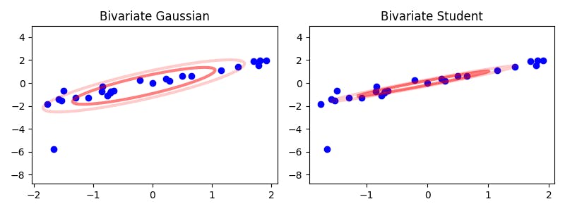
As the image also suggests, the Gaussian model can easily be thrown off by a small number of very extreme observations. If we extract a linear model from the estimated parameters, we will therefore get much more robust estimates when we use the multivariate t distribution.

Image credit: the cover image is taken from the Louisiana Governor's Office of Homeland Security and Emergency Preparedness and shows oil washing ashore after the Deepwater Horizon oil spill. The remaining illustrations are mine.