
The HSV color model parameterizes the pure colors in terms of angles. While the idea of using an angle to select a point on a color wheel is intuitive enough, the precise mapping between angle and hues is somewhat involved. Since I recently understood the motivation behind the parameterization, I want to explain it here.
In the usual RGB model of the color space, every color of light is specified in terms of the amounts of red, green, and blue light it contains. A color can then be described by a point (r, g, b) in the unit cube, where 0 means no light of the given primary color, and 1 means the largest possible amount of light.
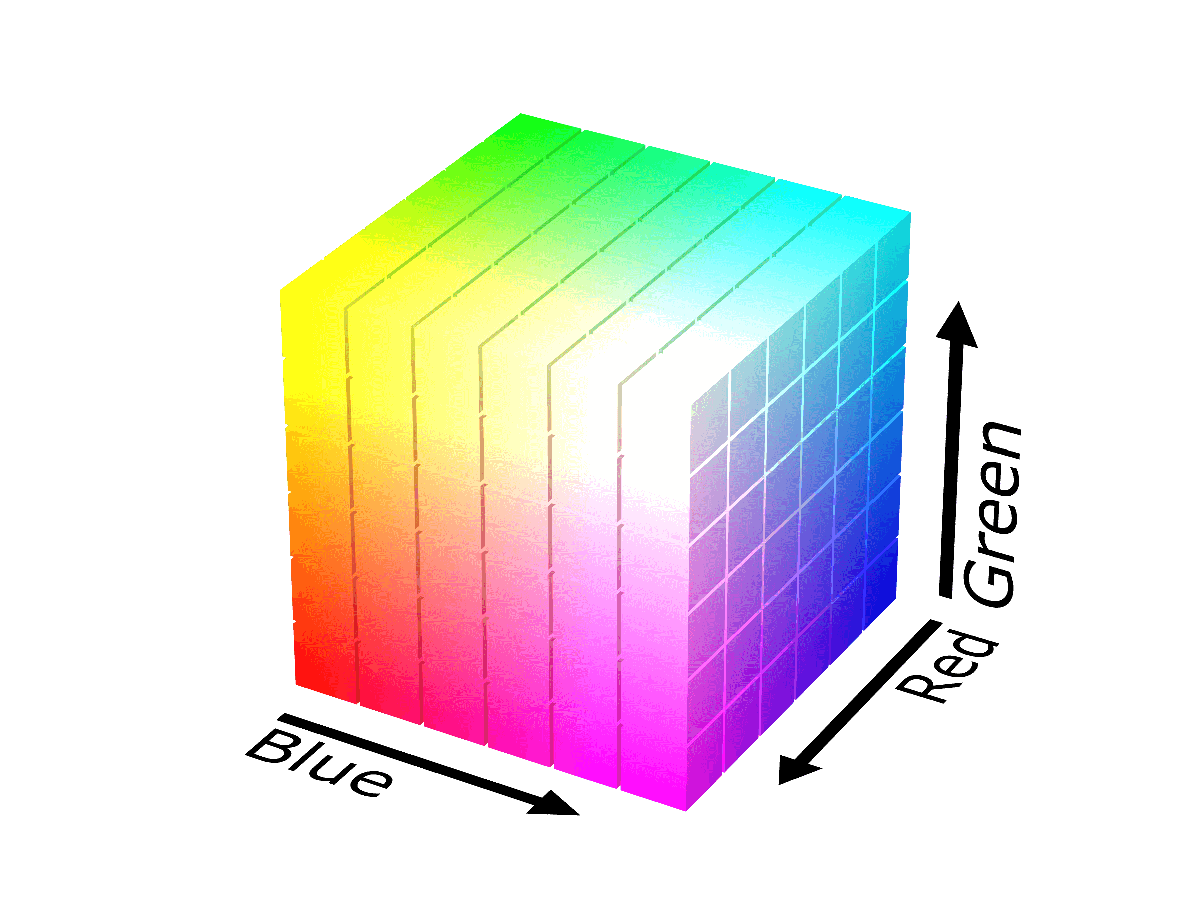
Inside the color cube, there is a diagonal connecting the corner points (0, 0, 0) and (1, 1, 1). These corners represent black and white, and points on the diagonal are the grayscale values. We might, therefore, be tempted to describe any color in terms of
"Saturation": the distance from the grayscale axis to the point
"Brightness": the distance from the point to the "black plane" orthogonal to the grayscale axis and passing through (0, 0, 0)
"Hue": the angle around the grayscale axis starting from an arbitrary reference point, such as a suitably bright red.
Sadly, there are some problems with this approach:
The distance from the grayscale axis to the edge of the color cube varies greatly for different values of r + g + b, so the proposed "saturation" would have different ranges depending on the brightness level.
If we rotate a highly saturated RGB color such as (r, g, b) = (1, 0, 0) around the grayscale axis, we may encounter non-valid RGB colors with coordinate values outside the unit interval.
The colors cyan, magenta and yellow would not be rotated versions of red, green, and blue (because cyan, magenta, and yellow all have r + g + b = 2, while red, green, and blue have r + g + b = 1).
For this reason, the HSV color model defines a rather exotic color wheel which is not actually a circle around the grayscale axis, but rather a piecewise linear zigzag path that goes straight from red to yellow to green to cyan to blue to magenta:
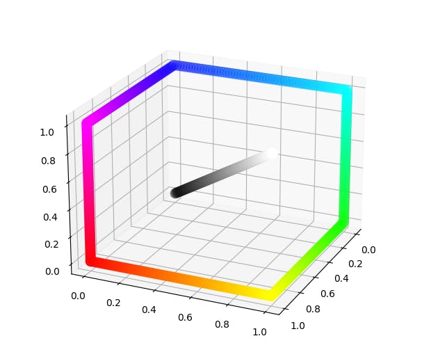
This is achieved by defining the brightness not as r + g + b but as max{r, g, b}. The set of colors of a given level of brightness is therefore not a plane through the grayscale axis, but the outer half of a cube (or, if you will, an L-infinity sphere).
This has the disadvantage that the mapping from HSV coordinates to RGB coordinates has several case distinctions. It has the advantage that all six reference colors (as well as white) count as maximally bright and maximally saturated.
By contrast, if we literally rotate the color red around the grayscale axis and truncate the result so it lies inside the color cube, then we can obtain the pure colors green and blue, but not cyan, yellow, or magenta. Conversely, if we rotate the color yellow around the grayscale axis, we can obtain the colors cyan and magenta, but not red, green, or blue:
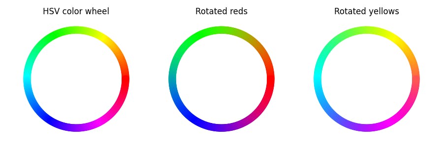
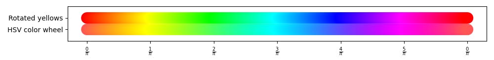
Note that while the HSV color wheel and the rotated yellows look very similar (and they coincide exactly at yellow, magenta, and cyan), they are subtly different:
The rotated reds appear dimmer than the two other color wheels. This observation is corroborated by the graphs of r + g + b for each of these color wheels:
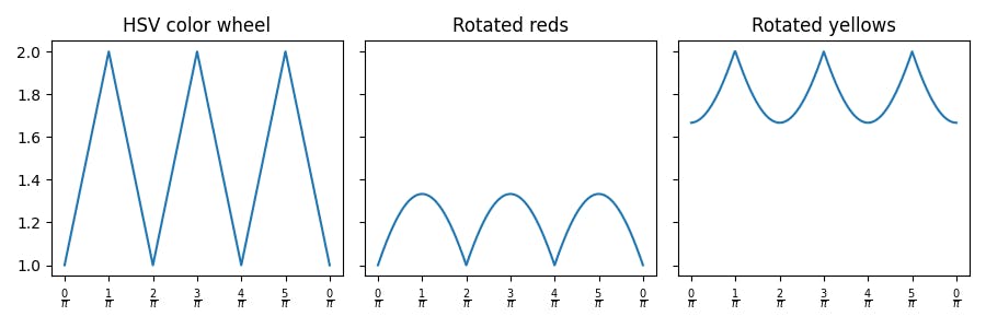
If instead we apply the HSV value, i.e., max{r, g, b}, then these three graphs instead look as follows:
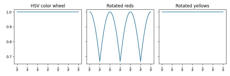
This confirms that the HSV color wheel contains only, by its own definition, maximally bright values.
Image credits: the cover image is an early color photograph by Sergei Prokudin-Gorskii; the picture of the RGB cube comes from the Wikipedia article about the RGB color model; the other pictures are by me.